我在Excel中为按行着色设定了以下条件格式规则：

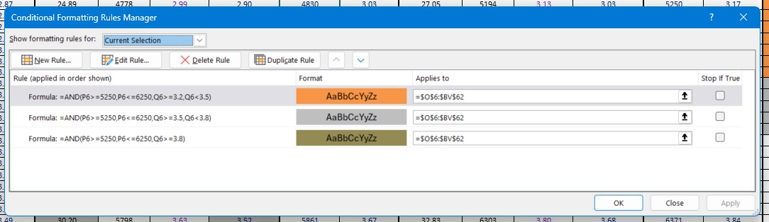
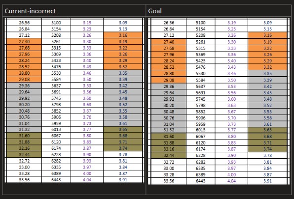
我希望颜色编码在重复序列中应用到第1到第4列中的每一列（不仅仅是第1列和第4列）。并且不太清楚为什么在并非满足所有条件时，某些会错位/偏移。应该像下面这样显示（手动修正后的列集合并标出边框）：

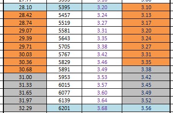
下面是另一张截图。我希望蓝色行的格式与橙色和灰色的格式一致，但似乎它没有扩展到其他列

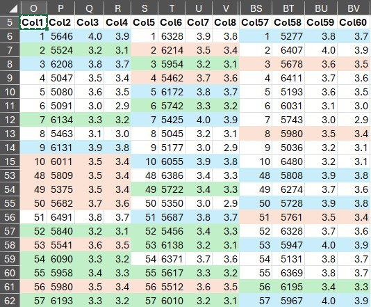
解决方案

应用多重条件格式

Sub ApplyMultipleCF()

    ' Define constants.
    Const SHEET_NAME As String = "Sheet1"
    Const COLUMN_SETS_SIZE As Long = 4
    Const TOTAL_RANGE_ADDRESS As String = "O6:BV62"
    Const COL1 As Long = 2 ' column of Cell1
    Const COL2 As Long = 3 ' column of Cell2
    ' The following two need to be 'in sync'.
    Dim FORMAT_COLORS() As Variant: FORMAT_COLORS = VBA.Array( _
        13168833, 14017275, 16510410) ' green, red, blue
    Dim FORMAT_CONDITIONS() As Variant: FORMAT_CONDITIONS = VBA.Array( _
        "=AND(Cell1>=5250,Cell1<=6250,Cell2>=3.2)", _
        "=AND(Cell1>=5250,Cell1<=6250,Cell2>=3.5)", _
        "=AND(Cell1>=5250,Cell1<=6250,Cell2>=3.8)")

    ' Reference the objects (workbook, worksheet, and range).
    Dim wb As Workbook: Set wb = ThisWorkbook ' workbook containing this code
    Dim ws As Worksheet: Set ws = wb.Sheets(SHEET_NAME)
    Dim rg As Range: Set rg = ws.Range(TOTAL_RANGE_ADDRESS)

    ' Retrieve the number of columns.
    Dim ColumnsCount As Long: ColumnsCount = rg.Columns.COUNT

    ' Calculate (and validate) the number of sets.
    Dim SetsCalculated As Double:
    SetsCalculated = ColumnsCount / COLUMN_SETS_SIZE
    If SetsCalculated - Int(SetsCalculated) <> 0 Then
        MsgBox "The number of columns (" & ColumnsCount & ") " _
            & "is not divisible by the number of column sets size (" _
            & COLUMN_SETS_SIZE & ")!", vbExclamation
        Exit Sub
    End If
    Dim SetsCount As Long: SetsCount = SetsCalculated

    ' Clear all existing conditional formatting.
    ws.Cells.FormatConditions.Delete

    ' Apply conditional formatting.

    Dim srg As Range, n As Long, i As Long
    Dim Cell1 As String, Cell2 As String, CFormula As String

    For n = 1 To SetsCount
        Set srg = rg.Resize(, COLUMN_SETS_SIZE) _
            .Offset(, (n - 1) * COLUMN_SETS_SIZE)
        With srg
            Cell1 = .Cells(1, COL1).Address(0) ' lock column
            Cell2 = .Cells(1, COL2).Address(0) ' lock column
            For i = 0 To UBound(FORMAT_CONDITIONS)
                CFormula = Replace(FORMAT_CONDITIONS(i), "Cell1", Cell1)
                CFormula = Replace(CFormula, "Cell2", Cell2)
                With .FormatConditions.Add(Type:=xlExpression, _
                        Formula1:=CFormula)
                    .SetFirstPriority
                    .Interior.Color = FORMAT_COLORS(i)
                    '.StopIfTrue = True ' default
                End With
            Next i
        End With
    Next n

    MsgBox "Conditional formattings applied.", vbInformation

End Sub

备选方案

你也可以在不使用VBA的情况下实现类似的结果，但需要定义一些名称来指定相关列的地址。例如，如果格式化范围从第 O 列开始（第15列），你可以在 Name Manager 中定义两个名称：
scol : =INDIRECT("RC"&4*INT((COLUMN()-15)/4)+15+1,FALSE)
tcol : =INDIRECT("RC"&4*INT((COLUMN()-15)/4)+15+2,FALSE)
或者，你也可以使用以下名称：
scol : =OFFSET($O6,,4*INT((COLUMN()-15)/4)+1)
tcol : =OFFSET($O6,,4*INT((COLUMN()-15)/4)+2)
因为最后两个名称包含明确的相对行引用，在你定义这些名称时活动单元格应该位于第六行（或者你应该在名称定义中使用正确的行号）。
现在我们按与提问者使用的相同方式来定义格式条件：
=AND(scol >= 5250, scol <= 6250, tcol >= 3.2, tcol < 3.5)
=AND(scol >= 5250, scol <= 6250, tcol >= 3.5, tcol < 3.8)
=AND(scol >= 5250, scol <= 6250, tcol >= 3.8)