我有一个Excel工作簿，有时需要把其中选定的一些工作表复制到一个新文件中。

为此，我在一个示例文件中编写了以下宏：

Sub Copy_to_new_workbook()


    Sheets(Array("Blad1", "Blad2", "Blad3", "Blad4", "Blad5", "Blad6", "Blad7", "Blad8", _
        "Blad9", "Blad10", "Blad11", "Blad12", "Blad13", "Blad14", "Blad15", "Blad16", "Blad18" _
        , "Blad20", "Blad21", "Blad22", "Blad23", "Blad24", "Blad25", "Blad26", "Blad27", _
        "Blad28", "Blad30", "Blad32", "Blad33", "Blad34")).Copy
' copy the sheets Blad1 through Blad34 to a new workbook,
' skipping Blad17, Blad19, Blad29 and Blad31

' Anything that happens from here would be done in the newly created workbook.
' This also involves selecting every sheet and pasting all data therein as values.
' Thus, another block of "Sheets(Array([all of the above again])).Select" would appear in the macro here.


End Sub

上面的代码块是Excel的“记录宏”功能的结果，事后已把不必要的操作去掉。
虽然这段代码（以及注释段中提到的所有内容）确实能工作，但长期可用的、较长的版本在需要向这个数组中添加新工作表时会比较难维护；毕竟该文件的工作表名称并非简单的连续命名。
我过去曾通过重新从头录制宏来解决，但现在这也越来越困难。上次我尝试用这种方式更新实时文件时，在对所选工作表右键点击以复制它们时，Excel会持续冻结，无论等待多久都无法自行恢复。只有在“录制宏”期间才会发生这种情况。录制模式之外，这一步就能立即完成。

我个人觉得Excel的公式比VBA更容易阅读和维护，因此我想把宏中硬编码的工作表名称数组替换为一个变量，从数组公式中读取。我为此准备了以下内容：

工作簿中的每个工作表在M2单元格都有一个公式，用来返回该工作表的名称。
=TEXTAFTER(CELL("filename",$A$1),"]")
对于需要复制的所有工作表，这些名称在工作簿总览表的E8#的数组公式中一起列出。
=VSTACK(Blad1:Blad16!$M$2,Blad18!$M$2,Blad20:Blad28!$M$2,Blad30!$M$2,Blad32:Blad34!$M$2)

我尝试了 这个解决方案，以在VBA中定义数组公式的输出。把其中一部分逐字拷贝，在宏开头放了如下代码：

Dim DirArray As Variant 
DirArray = Range("E8", Range("E8").End(xlDown)).Value

据我所知，来自E8#的数据已经正确保存到DirArray。

这就是我卡在这一步的地方。把代码块剩下的部分缩短为 Sheets(DirArray).Copy 或 Sheets(Array(DirArray)).Copy 会返回类型不匹配的错误。为了让DirArray能以工作表名称的列表被VB读取，我应该怎么做？

解决方案

如果你愿意接受一种略有不同的做法。这个方法会复制所有工作表，除了排除列表中的工作表。

下面是一个Excel表格（VBA ListObject），我把它命名为 SkipSheets。

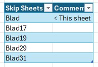
Public Sub CopySheets()

    'Create a workbook containing a single sheet.
    Dim wrkbk As Workbook
    Set wrkbk = Workbooks.Add(xlWBATWorksheet)

    'Get reference to sheet names **not** to include.
    Dim SkipSheet As Range
    With ThisWorkbook.Worksheets("Blad").ListObjects("SkipSheets")
        If Not .DataBodyRange Is Nothing Then
            Set SkipSheet = .ListColumns("Skip Sheets").DataBodyRange
        End If
    End With

    'Look at each sheet in turn.
    Dim wrksht As Worksheet
    For Each wrksht In ThisWorkbook.Worksheets
        'Is the sheet in the exclusion list?
        Dim ExcludeSheet As Range
        Set ExcludeSheet = SkipSheet.Find(What:=wrksht.Name, _
                                          After:=SkipSheet.Cells(1, 1), _
                                          LookIn:=xlValues, _
                                          LookAt:=xlWhole, _
                                          SearchOrder:=xlByRows, _
                                          SearchDirection:=xlNext, _
                                          MatchCase:=False)

        If ExcludeSheet Is Nothing Then
            Dim rLastCell As Range
            Set rLastCell = LastCell(wrksht)

            'Use Sheets.Count rather than Worksheets.Count so Charts sheets are included.
            Dim NewSht As Worksheet
            Set NewSht = wrkbk.Worksheets.Add(After:=wrkbk.Sheets(wrkbk.Sheets.Count))
            NewSht.Name = wrksht.Name

            'Copy the range containing data.
            wrksht.Range(wrksht.Cells(1, 1), rLastCell).Copy

            'Use PasteSpecial to add the data to the new sheet.
            With NewSht.Range("A1")
                .PasteSpecial Paste:=xlPasteValuesAndNumberFormats
                .PasteSpecial Paste:=xlPasteFormats
                .PasteSpecial Paste:=xlPasteColumnWidths
            End With
        End If
    Next wrksht

    'Remove the first sheet.
    Application.DisplayAlerts = False
    wrkbk.Worksheets(1).Delete
    Application.DisplayAlerts = True

End Sub

'Returns a reference to the last cell containing data on the specified worksheet.
Public Function LastCell(wrksht As Worksheet) As Range
    Dim lLastCol As Long, lLastRow As Long
    On Error Resume Next
        With wrksht
            lLastCol = .Cells.Find("*", , xlValues, xlWhole, xlByColumns, xlPrevious).Column
            lLastRow = .Cells.Find("*", , xlValues, xlWhole, xlByRows, xlPrevious).Row
        End With
        If lLastCol = 0 Then lLastCol = 1
        If lLastRow = 0 Then lLastRow = 1
        Set LastCell = wrksht.Cells(lLastRow, lLastCol)
    On Error GoTo 0
End Function

备选方案

感谢 @CDP1802在评论中的回答：

Range("E8", Range("E8").End(xlDown)).Value 返回一个 2-D 数组，元素为 DirArray(1,1), DirArray(2,1) 等等。Array("Blad1", "Blad2" 等是一维，元素为 DirArray(0), DirArray(1) 等等。使用 Sheets(Application.Transpose(DirArray)).Copy。Transpose() 将二维列转换为一维行。

我之前并不知道它其实是一个二维数组，直接应用 Application.Transpose() 就能立即起效。我按照如下实现：

DirArray = Application.Transpose(Range("E8", Range("E8").End(xlDown)).Value)
Sheets(DirArray).Copy