我在R 中使用simr进行线性混合模型分析的功效计算。我想弄清楚，为什么通过改变人工数据集的结构，会出现完全不同的功效。在一种情况下，功效为0%；在另一种情况下，功效超过80%。

我计划一个组间-组内混合设计。有两个组（年龄分组：Y与 O）。每组中的每个人都在两种呼吸条件下进行观测。我构建了一个人工数据集，其中包含呼吸条件、年龄分组和1000个 ID。ID的一半来自Y 组，另一半来自O 组。ID被存储为因子变量。

我沿着ID运用powerCurve，以估计在40、60、80、和100个 ID水平下检测年龄分组与呼吸处理之间的交互效应的功效。

最初，我将数据结构化为所有属于Y 组的ID先排在前面，其次是来自O 组的ID。这样做时，我得到的功效为0%。

这就是功效的样子：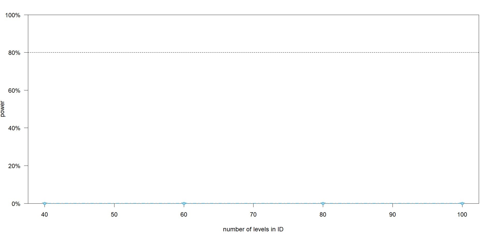

这是我的代码：

## generate artificial data-set
n_participants <- 1000L
n_trials <- 16L

## 1. create artificial dataset incl ID, Trial, breathing manipulation
artificial_data <- expand.grid(
  trial_total=seq_len(n_trials),
  breathing_manipulation=factor(c('spontaneous', 'slow-paced')),
  id=factor(seq_len(n_participants))
)

# 2. create variable agegroup
age_group <- factor(
  c(rep('Y', n_trials*1000),
    rep('O', n_trials*1000))
) ## considering n participants, trials, 2 conditions

## 3. combine artificial dataset with agegroup
artificial_data <- cbind(artificial_data, age_group)
str(artificial_data)

## 4. set reference level of breathing manipulation and agegroup
artificial_data$breathing_manipulation <- relevel(
  artificial_data$breathing_manipulation,
  'spontaneous'
)
artificial_data$age_group <- relevel(artificial_data$age_group, 'Y')
str(artificial_data)

col_order <- c('id', 'age_group', 'breathing_manipulation',
               'trial_total')
artificial_data2 <- artificial_data[, col_order]
rm(artificial_data)
artificial_data <- artificial_data2
rm(artificial_data2)
str(artificial_data)

## create model
vars <- 0.51
res <- 0.7
fixed_intercept_only <- 0.001374236
beta_age <- 0.30
beta_interaction <- 0.24
fixed_breathing_manipulation <- 0.0001

fixed_full <- c(
  fixed_intercept_only,
  beta_age,
  fixed_breathing_manipulation,
  beta_interaction
)

library(simr)

simulated_model_full <- makeLmer(
  z_score ~ 1 + age_group*breathing_manipulation + (1 | id),
  fixef=fixed_full,
  VarCorr=vars,
  sigma=res,
  data=artificial_data
)

p_curve_hp <- powerCurve(
  simulated_model_full,
  test=fcompare(z_score ~ breathing_manipulation),
  along='id',
  breaks=c(40, 60, 80, 100),
  alpha=0.05
)

plot(p_curve_hp)

我现在将它的结构改为在group列下的ID顺序为：Y、O、Y、O。随后获得了一个相对合理的功效。

这是创建 age_group 的新代码：

age_group <- factor(
  rep(
    c(rep('Y', n_trials*2),
      rep('O', n_trials*2)),
    n_participants/2
  )
)

现在的功效看起来是这样的：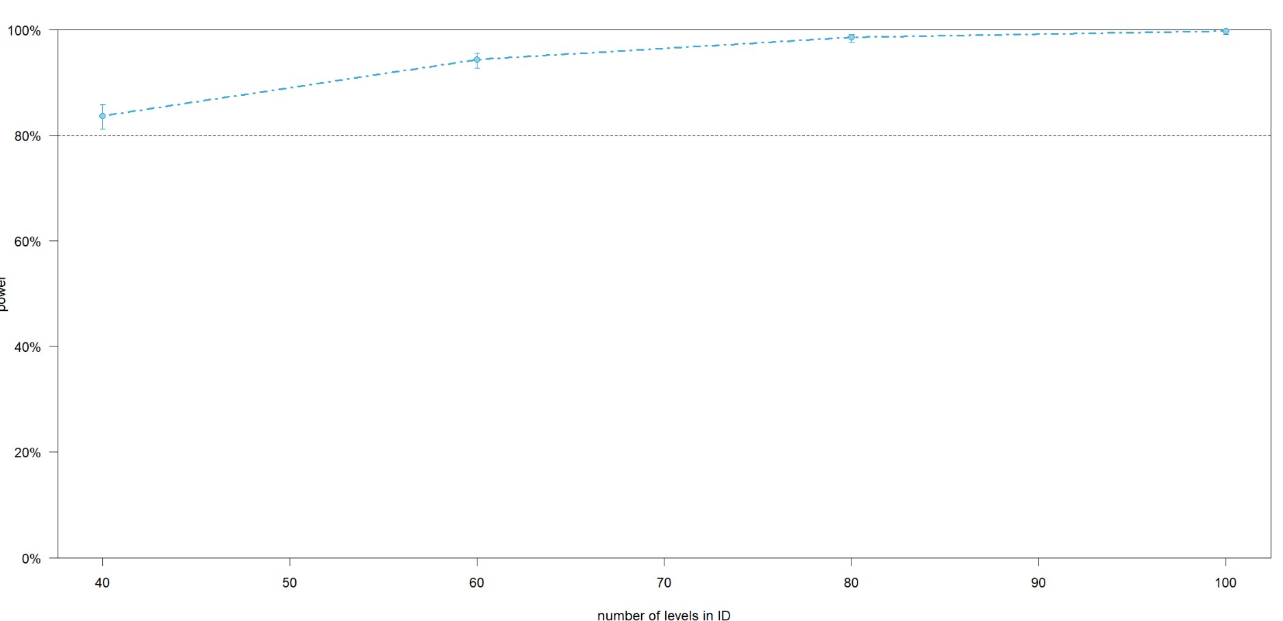

你能告诉我为什么会这样吗？我对如何组织这段代码的理解正确吗？

解决方案

你的 age_group 本质上是对的，只是让它写得更明确、不要那么硬编码：

age_group <- factor(
  rep(c('Y', 'O'), each=n_trials*2, length.out=nrow(artificial_data))
)

然而，为了测试交互作用，通常将完整模型与仅去除了交互作用、保留主效应的简化模型进行比较

full = z_score ~ age_group*breathing_manipulation + (1 | id)

与一个仅去除了交互作用、保留主效应的简化模型对比

red = z_score ~ age_group + breathing_manipulation + (1 | id)

同时去掉年龄分组的主效应也会测试一个更广泛的对比，可能会让交互效应的功效略显乐观。

下面给出一个更快的替代方法，替代 simr，它反复执行 refits、full 与 red，使用带有模拟响应（随机截距和残差噪声）的数据来评估似然比，通过 anova() 来实现：

one_power_n <- \(n_id, B=1000L, beta=fixed_full, tau=.51, sigma=.7,
                 n_cores=parallel::detectCores() - 1L) {
  ids <- levels(artificial_data$id)[seq_len(n_id)]
  dat <- artificial_data[artificial_data$id %in% ids, ]
  dat$id <- droplevels(dat$id)
  dat$z_score <- 0
  full <- lme4::lmer(z_score ~ age_group*breathing_manipulation + (1 | id),
                     dat, REML=FALSE)
  red <- lme4::lmer(z_score ~ age_group + breathing_manipulation + (1 | id),
                    dat, REML=FALSE)
  # red <- lme4::lmer(z_score ~ breathing_manipulation + (1 | id),
  #                   dat, REML=FALSE)
  x <- model.matrix(~ age_group*breathing_manipulation, dat)
  id_i <- as.integer(dat$id)
  p <- pbmcapply::pbmclapply(seq_len(B), \(i) {
    y <- drop(x %*% beta) +
      rnorm(n_id, 0, sqrt(tau))[id_i] +  ## random intercept
      rnorm(nrow(dat), 0, sigma)  ## residual noise
    anova(lme4::refit(red, y), lme4::refit(full, y))$`Pr(>Chisq)`[2L]
  }, mc.cores=max(1L, n_cores))
  p <- unlist(p, use.names=FALSE)
  n_ok <- sum(!is.na(p))
  pow <- mean(p < .05, na.rm=TRUE)
  data.frame(n_id=n_id, nsim=n_ok, power=pow, se=sqrt(pow*(1 - pow)/n_ok))
}

ns <- c(40L, 60L, 80L, 100L)
power_tab <- do.call(rbind, lapply(ns, one_power_n))

注： 这使用 pbmclapply()，因此适用于类Unix的系统。在Windows上，请改用通过 parallel::makeCluster() 的PSOCK集群。

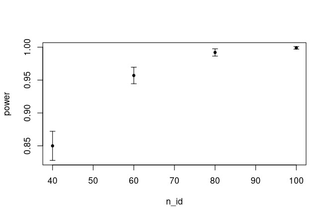
结果为

> power_tab
  n_id nsim power           se
1   40 1000 0.850 0.0112915898
2   60 1000 0.957 0.0064149045
3   80 1000 0.992 0.0028170907
4  100 1000 0.999 0.0009994999

如果你使用被注释掉的“乐观”简化模型（去掉年龄组和交互），结果将与你当前的估计保持一致。

绘图

z <- qnorm(.975)

ylim <- with(
  power_tab,
  range(pmin(1, pmax(0, power + z*c(-se, se))))
)

plot(power ~ n_id, power_tab, ylim=ylim, pch=20)

with(power_tab,
     arrows(n_id, power - z*se, n_id, power + z*se,
            angle=90, code=3, length=.05)
)