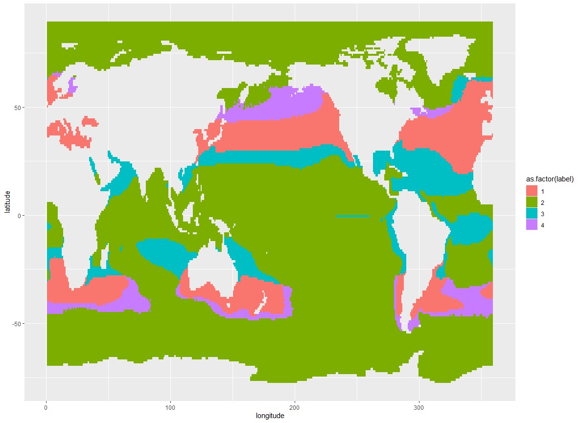
我正在尝试基于数据中的标签变量，通过 geom_tile() 在地图上为不同的颜色着色。

library(rnaturalearth) 
library(ggplot2)
library(sf)
library(dplyr)

T_Fe_0.6 <- read.csv("T_Fe_0.6.csv")
ggplot()+
  geom_tile(data = T_Fe_0.6,aes(x = longitude,y = latitude,fill = as.factor(label)))

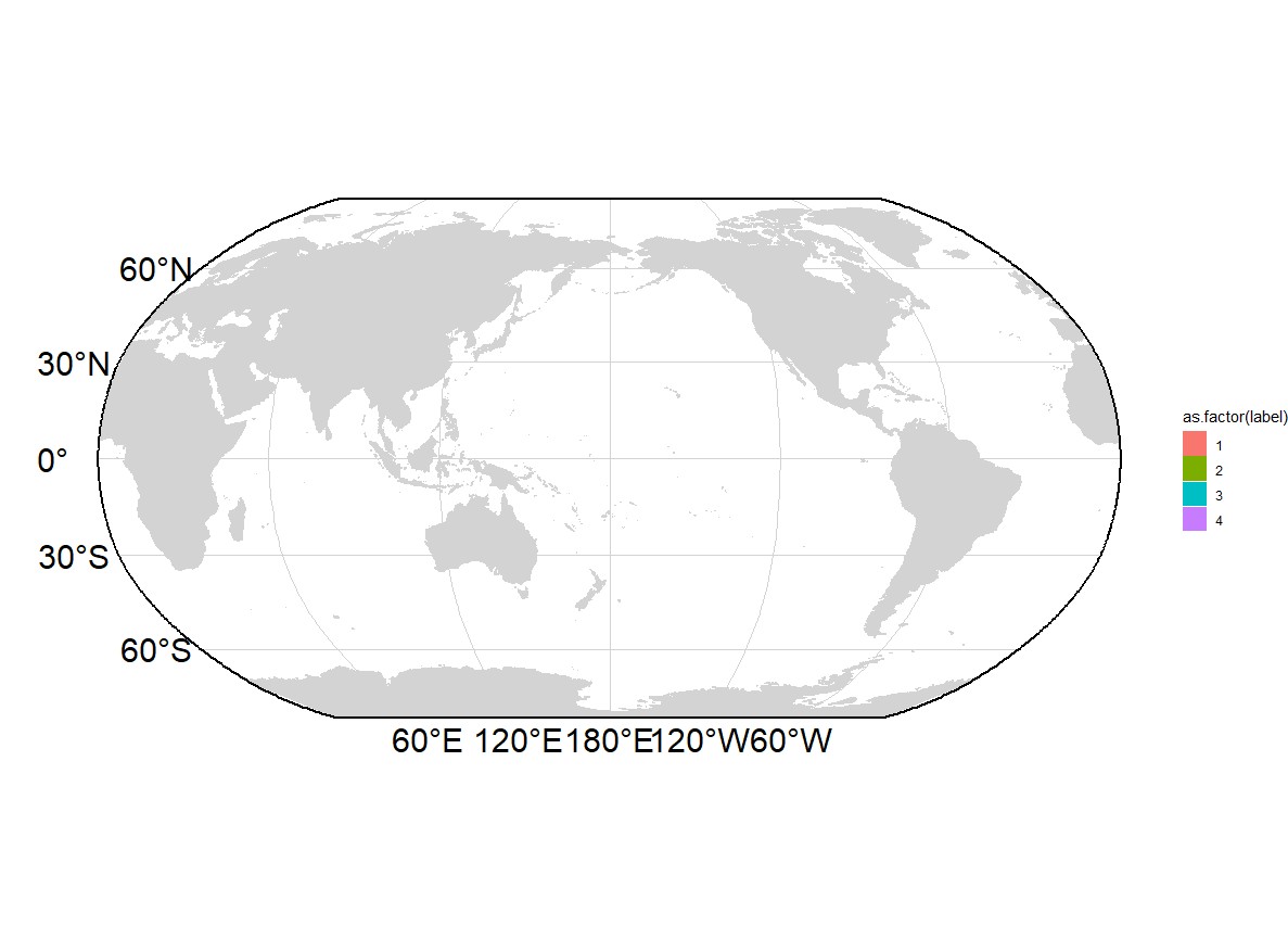
当我添加了一些美观的图层，它们使用一个自定义的Robinson投影CRS，颜色就消失了。这似乎与投影有关。

world <- ne_countries(scale = "medium", returnclass = "sf")

world <- world |> 
  st_break_antimeridian(lon_0 = 180) |> 
  st_transform(crs = "+proj=robin +lon_0=180 +x_0=0 +y_0=0 +ellps=WGS84 +datum=WGS84 +units=m +no_defs")

lats <- seq(-90, 90, by = 1)
lons_left <- rep(-0.001, length(lats))
lons_right <- rep(360.001, length(lats))

border_coords <- rbind(
  cbind(lons_right, lats),
  cbind(rev(lons_left), rev(lats))
)
border_coords <- rbind(border_coords, border_coords[1, ])

border <- suppressWarnings(
  st_polygon(list(border_coords)) |>
    st_sfc(crs = 4326) |>
    st_segmentize(100000) |>
    st_transform("+proj=robin +lon_0=180 +x_0=0 +y_0=0 +ellps=WGS84 +datum=WGS84 +units=m +no_defs")
)

grat <- st_graticule(x = c(0,-90,360,90),crs = 4326, lon = c(60,120,180,240,300),
                     lat = seq(-90,90,by = 30)) |> 
  filter(plot12 == "TRUE")

# lon
labels_x_init <- grat |> 
  filter(type == "E") |> 
  mutate(lab = ifelse(degree > 180,paste0(360-degree,"°W"),
                      paste0(degree, "°E")))
labels_x <- st_as_sf(st_drop_geometry(labels_x_init), lwgeom::st_startpoint(labels_x_init))

# lat
labels_y_init <- grat |> 
  filter(type == "N") |> 
  mutate(lab = ifelse(degree == 0, "0°",
                      ifelse(degree > 0, paste0(degree, "°N"),
                             paste0(-degree, "°S"))))

labels_y <- st_as_sf(st_drop_geometry(labels_y_init), lwgeom::st_startpoint(labels_y_init))

ggplot()+
  geom_tile(data = T_Fe_0.6,aes(x = longitude,y = latitude,fill = as.factor(label)))+
  geom_sf(data = world, fill = "lightgrey", color = "lightgrey")+
  geom_sf_text(data = labels_x, aes(label = lab), nudge_y = -0.7e6, size = 8)+
  geom_sf_text(data = labels_y, aes(label = lab), nudge_x = -1.5e6, size = 8)+
  geom_sf(data = grat, color = "lightgrey", linewidth = 0.3)+
  geom_sf(data = border, fill = NA, color = "black", linewidth = 1) +
  theme_void()

T_Fe_0.6.csv下载链接.

解决方案

在处理空间数据时，几乎总是 最好确保所有绘图对象都具备空间引用。这在使用像Robinson或 Mollweide这样的非保形CRS时尤为如此。这有助于避免你所遇到的问题。

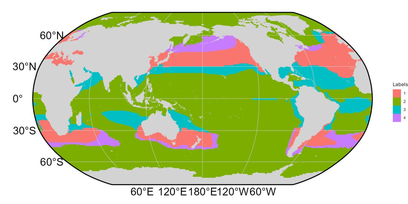
除了纠正你的 st_graticule() 代码外，这个方案还模仿 geom_tile()。它的工作原理是先将你的数据框转换为具备空间引用的SpatRaster。假设T_Fe_0.6的坐标是WGS84/EPSG:4326。你所有其他代码保持不变。

terra 包用于创建SpatRaster，tidyterra::geom_spatraster() 函数是绘制SpatRaster所必需的。要让这段代码工作，你需要同时安装这两个包。

还有一个需要考虑的点是，你的T_Fe_0.6数据并没有“整齐地”覆盖到Natural Earth多边形的外接范围。这会在某些位置留下空白区域，尤其是在南极周围。就南极而言，Natural Earth数据并不包含冰架的完整范围，而你的数据似乎在此处停止。我提供了一个替代方法，使用多边形来填充背景。如果你需要保留空白区域，可以省略。

library(rnaturalearth)
library(sf)
library(dplyr)
library(terra)
library(tidyterra)
library(ggplot2)

# Define PROJ4 projection string variable
robin_prj <- "+proj=robin +lon_0=180 +x_0=0 +y_0=0 +ellps=WGS84 +datum=WGS84 +units=m +no_defs"

# st_graticule() object with correctly declared CRS
grat <- st_graticule(
  x = c(0, -90, 360, 90),
  crs = st_crs(4326),
  lon = c(60, 120, 180, 240, 300),
  lat = seq(-90, 90, by = 30)
  ) |> 
  filter(plot12)

# Create SpatRaster version of T_Fe_0.6, WGS84 is assumed
r <- rast(
  T_Fe_0.6[, c("longitude", "latitude", "label")],
  crs = "EPSG:4326"
  )

# Convert numeric 'label' values to strings, which achieves 
# the equivalent of as.factor(label) in your code
r[] <- as.character(r[])

# Create 'background' sf polygon using WGS84 extent,
# then project to robin_prj
bbox <- st_as_sfc(
  st_bbox(c(xmin = 0,
            ymin = -89.99,
            xmax = 359.99,
            ymax = 90),
          crs = 4326)) %>%
  st_segmentize(1e5) %>% 
  st_transform(robin_prj)

# Plot
ggplot() +
  geom_sf(data = bbox, fill = "lightgrey", color = "lightgrey") +
  geom_spatraster(data = r, aes(fill = label)) +
  scale_fill_discrete(
    name = "Labels",
    na.value = "transparent",
    na.translate = FALSE
  ) +
  geom_sf(data = world, fill = "lightgrey", color = "lightgrey") +
  geom_sf_text(data = labels_x, aes(label = lab), nudge_y = -0.7e6, size = 8) +
  geom_sf_text(data = labels_y, aes(label = lab), nudge_x = -1.5e6, size = 8) +
  geom_sf(data = grat, color = "lightgrey", linewidth = 0.3) +
  geom_sf(data = border, fill = NA, color = "black", linewidth = 1) +
  theme_void()

为了可重复性，防止OP的数据链接失效，这里给出T_Fe_0.6的一个reprex版本：

T_Fe_0.6 <- data.frame(
  expand.grid(longitude = seq(0.99, 359, length.out = 360),
              latitude = seq(-77, 89, length.out = 118)),
  label = rep(1:4, each = 10620)
  )